Augmented Synthetic Difference-in-Differences (ASDID)
ASDID is a causal inference estimator for panel data that combines the strengths of Difference-in-Differences (DID) and Synthetic Control (SC) methods, building on the Synthetic Difference-in-Differences (SDID) framework by Arkhangelsky et al. (2021).
When to use ASDID
You have panel data (units observed over time) with a treatment that starts at a known time
Parallel trends may not hold exactly (some units are better controls than others)
You have many control units (100s to millions) and want to select the best donors
You need power analysis or inference via placebo tests
Key differences from SDID
Feature |
SDID |
ASDID |
|---|---|---|
Fixed effects |
Intercept in solver |
Two-way demeaning (explicit FE removal) |
Regularization |
|
MAD² of first-differences (data-driven, robust) |
Time weighting |
Equal weight per observation |
Inverse-variance weighting (downweights noisy periods) |
Scalability |
~1000 units (Frank-Wolfe) |
5M+ units (PGD + donor screening) |
Covariates |
Joint optimization |
Partial-out via FWL theorem |
Quick Start: Panel Estimator
The simplest way to use ASDID within the azcausal framework:
[1]:
from azcausal.data import CaliforniaProp99
from azcausal.estimators.panel.asdid import ASDID

# Load the California Proposition 99 dataset
panel = CaliforniaProp99().panel()

# Fit ASDID
result = ASDID().fit(panel)
print(result.summary())
╭──────────────────────────────────────────────────────────────────────────────╮
|                                    Panel                                     |
|  Time Periods: 31 (19/12)                                  total (pre/post)  |
|  Units: 39 (38/1)                                       total (contr/treat)  |
├──────────────────────────────────────────────────────────────────────────────┤
|                                     ATT                                      |
|  Effect: -14.60                                                              |
|  Observed: 60.35                                                             |
|  Counter Factual: 74.95                                                      |
├──────────────────────────────────────────────────────────────────────────────┤
|                                  Percentage                                  |
|  Effect: -19.48                                                              |
|  Observed: 80.52                                                             |
|  Counter Factual: 100.00                                                     |
├──────────────────────────────────────────────────────────────────────────────┤
|                                  Cumulative                                  |
|  Effect: -175.19                                                             |
|  Observed: 724.20                                                            |
|  Counter Factual: 899.39                                                     |
╰──────────────────────────────────────────────────────────────────────────────╯
Standalone Package
The standalone module has no dependencies on azcausal — only numpy and scipy. It can be copied into any project and used independently.
from azcausal.standalone.asdid import asdid, did, se_placebo, power_curve
Data Preparation
Convert a long-format DataFrame to the matrix inputs using df_to_matrix. It validates that treatment assignment is consistent (block treatment).
[2]:
from azcausal.standalone.asdid import df_to_matrix, asdid
from azcausal.data import CaliforniaProp99

# Get raw DataFrame
df = CaliforniaProp99().df()
print(df.head())

# Convert to matrix format
Y, n_pre, treat = df_to_matrix(df, time_col="Year", unit_col="State",
                               outcome_col="PacksPerCapita", treat_col="treated")
print(f"Y: {Y.shape}, n_pre: {n_pre}, n_treat: {treat.sum()}")

# Run ASDID directly
att, lambd, omega, donors = asdid(Y, n_pre, treat)
print(f"ATT: {att[0]:.2f}")
         State  Year  PacksPerCapita  treated
0      Alabama  1970       89.800003        0
1     Arkansas  1970      100.300003        0
2     Colorado  1970      124.800003        0
3  Connecticut  1970      120.000000        0
4     Delaware  1970      155.000000        0
Y: (31, 39), n_pre: 19, n_treat: 1
ATT: -14.60
Estimation
Both asdid() and did() return (att, lambd, omega, donors):
[3]:
import numpy as np
from azcausal.standalone.asdid import asdid, did

# Prepare data as numpy arrays
panel = CaliforniaProp99().panel()
Y = panel['PacksPerCapita'].values  # (n_time, n_units)
n_pre = 19  # 19 pre-treatment periods
treat = np.zeros(39, dtype=bool)
treat[2] = True  # California is the treated unit

# ASDID: learns optimal unit weights (omega) and time weights (lambda)
att, lambd, omega, donors = asdid(Y, n_pre, treat)
print(f'ASDID: ATT = {att[0]:.2f} packs per capita')

# DID: uniform weights (standard difference-in-differences)
att_d, lambd_d, omega_d, donors_d = did(Y, n_pre, treat)
print(f'DID:   ATT = {att_d[0]:.2f} packs per capita')
ASDID: ATT = -14.60 packs per capita
DID:   ATT = -27.35 packs per capita
Inference
Standard errors can be computed via:
Placebo (
se_placebo): Permutation-based, recommended for n_treat=1. Correct coverage.Jackknife (
se_jackknife): Analytical leave-one-out, fast. Requires n_treat ≥ 2.
Inference functions take an estimator object as the first argument, decoupling estimation from inference:
[4]:
from azcausal.standalone.asdid import ASDID as ASDIDEstimator, se_placebo, summary

# Create estimator object (holds configuration)
est = ASDIDEstimator(max_donors=10000)

# Placebo SE: permutes treatment assignment to estimate null distribution
se = se_placebo(est, Y, n_pre, treat, n_placebo=200)

# Print formatted summary with confidence intervals
res = asdid(Y, n_pre, treat, return_dict=True)
summary(Y, n_pre, treat, res, se=se, conf=90, title='California Prop 99')
╭──────────────────────────────────────────────────────────────────────────────╮
│                              California Prop 99                              │
├══════════════════════════════════════════════════════════════════════════════┤
│                                    Panel                                     │
│  Time Periods: 31 (19/12) total (pre/post)                                   │
│  Units: 39 (38/1) total (contr/treat)                                        │
│  Donors: 38                                                                  │
├──────────────────────────────────────────────────────────────────────────────┤
│                                     ATT                                      │
│  Effect (±SE): -14.60 (±9.1203)                                              │
│  Confidence Interval (90%): [-29.60 , 0.40]                                  │
│  Observed: 60.35                                                             │
│  Counter Factual: 74.95                                                      │
├──────────────────────────────────────────────────────────────────────────────┤
│                                  Percentage                                  │
│  Effect (±SE): -19.48 (±12.17)                                               │
│  Confidence Interval (90%): [-39.49 , 0.54]                                  │
│  Observed: 80.52                                                             │
│  Counter Factual: 100.00                                                     │
├──────────────────────────────────────────────────────────────────────────────┤
│                                  Cumulative                                  │
│  Effect (±SE): -175.19 (±109.44)                                             │
│  Confidence Interval (90%): [-355.21 , 4.83]                                 │
│  Observed: 724.20                                                            │
│  Counter Factual: 899.39                                                     │
╰──────────────────────────────────────────────────────────────────────────────╯
Power Analysis
Simulate experiments to determine statistical power at different effect sizes. Uses the control panel to generate random treatment assignments and inject known ATTs.
[5]:
from azcausal.standalone.asdid import power_curve, plot_power_curve, mde, DID
import matplotlib.pyplot as plt

# Compare power: ASDID vs DID
att_values = [-25, -20, -15, -10, -5, 0, 5, 10, 15, 20, 25]

df_asdid = power_curve(est, Y, n_pre, n_treat=5, att_values=att_values, n_samples=200)
fig, _ = plot_power_curve(df_asdid, title='ASDID Power Curve — California Prop 99')
plt.show()

# Minimum detectable effect
print(f'ASDID MDE (90% conf, 90% power): {mde(se, conf=90, power=0.9):.1f} packs')
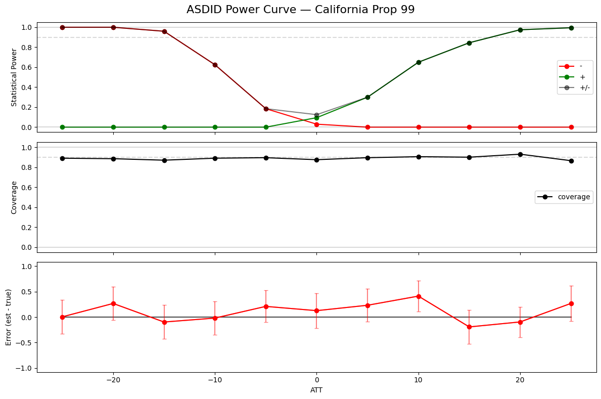
ASDID MDE (90% conf, 90% power): 26.7 packs
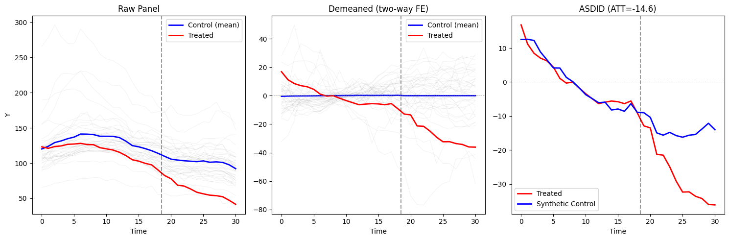
Visualization
Three-panel plot showing raw data, demeaned residuals, and the synthetic control fit:
[6]:
from azcausal.standalone.asdid import plot_asdid

res = asdid(Y, n_pre, treat, return_dict=True)
fig, _ = plot_asdid(Y, res)
plt.show()
Scalability
ASDID scales to millions of units via donor screening: an unconstrained ridge pre-screen identifies the top-K most relevant control units, then PGD optimizes weights on the reduced set.
[7]:
import time

# Generate a large panel: 500k units, 13 time periods
np.random.seed(42)
Y_big = np.random.randn(13, 500_000).astype(np.float32) * 0.5
Y_big[9:, -100:] += 3.0
treat_big = np.zeros(500_000, dtype=bool)
treat_big[-100:] = True

t0 = time.time()
att, lambd, omega, donors = asdid(Y_big, 9, treat_big, max_donors=1000)
elapsed = time.time() - t0

print(f'Panel: 500,000 units × 13 time periods')
print(f'ATT: {att[0]:.2f} (true: 3.0)')
print(f'Selected {len(donors)} donors from 499,900 controls')
print(f'Time: {elapsed:.2f}s')
Panel: 500,000 units × 13 time periods
ATT: 3.01 (true: 3.0)
Selected 1000 donors from 499,900 controls
Time: 0.09s
Covariate Adjustment
ASDID supports time-varying covariates via the Frisch-Waugh-Lovell theorem. Covariates are partialled out before weight estimation, removing confounding from observed factors that shift differently for treated and control units.
[8]:
# Example: covariates that confound the treatment effect
np.random.seed(42)
n_time, n_units, n_cov = 50, 30, 2
n_pre, n_treat = 35, 5
true_att, true_beta = 3.0, np.array([4.0, -2.5])

treat_ex = np.zeros(n_units, dtype=bool); treat_ex[-n_treat:] = True
X = np.random.randn(n_time, n_units, n_cov) * 0.5
X[n_pre:, -n_treat:, 0] += 1.5  # confounding covariate shift

Y_ex = np.random.randn(n_time, n_units) * 0.3
Y_ex += np.einsum('tnc,c->tn', X, true_beta)  # covariate effect
Y_ex[n_pre:, -n_treat:] += true_att

# Without covariates: biased
att_no_x, _, _, _ = asdid(Y_ex, n_pre, treat_ex)
# With covariates: corrected
att_with_x, _, _, _ = asdid(Y_ex, n_pre, treat_ex, X=X)

print(f'True ATT: {true_att}')
print(f'Without X: {att_no_x[0]:.2f} (biased by confounding)')
print(f'With X:    {att_with_x[0]:.2f} (corrected)')
True ATT: 3.0
Without X: 9.05 (biased by confounding)
With X:    3.10 (corrected)